Feature Discovery in Audio Models

I’ve been working on audio model interpretability as part of this year’s Mozilla Builders cohort. This post discusses the motivations behind my research, features I’ve discovered by inspecting intermediate activations in Whisper Tiny, features discovered with sparse autoencoders, and extending the work to larger Whisper models. You can find source code and instructions for replicating my work on Github, as well as pre-trained checkpoints and training logs on Huggingface.

TL;DR

• MLP neurons in Whisper tiny correspond well to interpretable features while also exhibiting polysemanticity, a result that can be checked at the hosted demo
• L1-regularized and TopK sparse autoencoders find interpretable features in the smallest and largest models in the Whisper family.

Readers familiar with mechanistic interpretability and SAEs and solely interested in this work’s novel results should read sections Analyzing MLP activations and Analyzing L1-regularized autoencoder for Whisper tiny through Looking for background noise features.

Background

The transformer architecture dominates the contemporary machine learning landscape due to its remarkable scaling properties, vindicated to great public acclaim when simply increasing the dataset size and the number of trainable parameters in GPT-2’s architecture produced the noticeably more capable GPT-3.

GPT-3’s success begged the question of whether the same transformer-scaling trick could apply to tasks other than text prediction. Two years later, OpenAI released Whisper, a family of speech-to-text models ranging in size from 39 million to 1.5 billion parameters. The training dataset contained 680,000 hours of audio, over 20 times the size of the largest dataset in prior published work.

Whisper is more capable than any speech-to-text program whose internal logic was explicitly set by a human. Still, the fact that Whisper’s transcription ability emerged by gradually updating millions of internal variables over hundreds of thousands of examples poses a disadvantage in understanding how the model makes the transcription decisions that it does. We can understand when a human-designed speech-to-text program outputs “dog” instead of “log” by inspecting the source code. However, if you look for the same information in Whisper’s model weights it’s hard to tell where the relevant dog/log information would be.

But how much do we care about understanding Whisper’s precise dog/log disambiguation procedure? We might care about deciphering the internal workings of powerful language models like GPT-3 and its successors to prevent them from generating incorrect content or understanding the mechanics underpinning generalized problem-solving and creativity. But why sweat the details of something as comparatively low-stakes as speech transcription?

whisper-large-v3 received over 4 million downloads in the month I wrote this blog post (November 2024), and as a matter of principle, we should try to understand how any program deployed that widely works. 

On a broader scope, work on understanding audio models lags behind work understanding text models despite other work on integrating the two: OpenAI recently rolled out Voice Mode for ChatGPT, and the open-source community responded with speech-comprehending local models such as this one that use Whisper to encode audio input. 

In light of indications that voice modality opens new avenues for provoking undesirable LLM behavior, understanding audio models proves more valuable than it may initially seem.

Mechanistic interpretability

Chris Olah analogizes the parameter-soup in the screenshot above to compiled bytecode. 

“Taking this analogy seriously can let us explore some of the big picture questions in mechanistic interpretability. Often, questions that feel speculative and slippery for reverse engineering neural networks become clear if you pose the same question for reverse engineering of regular computer programs. And it seems like many of these answers plausibly transfer back over to the neural network case.

Perhaps the most interesting observation is that this analogy seems to suggest that finding and understanding interpretable neurons – analogous to understanding variables in a computer program – isn’t just one of many interesting questions. Arguably, it’s the central task.”

Bytecode is optimized for computer execution, not human understanding; nevertheless, we can inspect program variables and execution behavior to recover an idea of the original human-comprehensible source code compiled into that bytecode. Likewise, we can look for “features” in neural networks that correspond to some meaningful concept and observe how manipulating these features affects network output to understand the task-relevant algorithms that the network developed during training.

Seeking linear features

It would be especially convenient if the neural network features we discovered formed a linear space over the network computations, given that linear spaces (aka vector spaces) have the following properties:

• The sum of two vectors is another vector in the space
• Any vector multiplied by a scalar is another vector in the space
• Every vector in the space can be decomposed into the sum of a collection of scalar-multiplied “basis vectors”
• Addition and scalar multiplication commute and distribute over the basis representation

These properties are nice because they allow us to go from reasoning about the entire space to just reasoning about the basis vectors. Since each vector and its transformations can be represented in terms of the basis, understanding the basis lets you interpret any vector in the space.

In a language model like GPT-3, finding vectors that correspond to human-comprehensible concepts and combine to form the model’s intermediate representations would provide insight into the model’s internal logic (“ah, the output “cats are annoying” comes from the sum of the features for “feline,” “domestic animal,” and “negative sentiment””) and allow us to manipulate it  (“let’s multiply the “negative sentiment” feature in the sum by -1, so that the output becomes “cats are adorable”). In an audio model like Whisper’s, we’d instead look for audio signals like phonemes or volume changes.

But the output of every intermediate layer of a transformer model is already a vector, isn’t it? A Pytorch tensor is a matrix of floating-point numbers, and the collection of such matrices forms a vector space equipped with a natural basis. Is it too much to hope that such basis vectors correspond to comprehensible feature-directions?

Where are the features?

The Whisper architecture follows the standard encoder-decoder format:

Since the decoder attends to both encoded audio and text tokens, we’ll focus our analysis on the encoder for simplicity. Here’s a look at the architecture of a transformer encoder block in isolation:

For a given encoder block, the activations that we could inspect are:

• The “residual stream” (the block’s final output, consisting of the sum of the input to the block with the output of the previous block layers)
• In the self-attention layer:
  • The final attention layer output
  • Query, key, and value embeddings
  • Attention head activations
• In the MLP (aka “feed-forward network”) layer:
  • The final MLP layer output
  • Intermediate MLP sublayer activations

If we’re hoping for particular activation coordinates to reliably correlate with semantic features (Anthropic’s interpretability writing calls this a privileged basis), we should exclude the residual stream from consideration:

Every layer performs an arbitrary linear transformation to “read in” information from the residual stream at the start. It then performs another arbitrary linear transformation before adding to “write” its output back into the residual stream. This linear, additive structure of the residual stream has many important implications. One basic consequence is that the residual stream doesn’t have a “privileged basis”; we could rotate it by rotating all the matrices interacting with it without changing model behavior.

In practice, residual stream occasionally does exhibit a privileged basis, but this derives not from the structure of the network itself but the fact that some commonly-used optimizers use coordinate-wise gradient statistics. Anyway, the logic above applies to most of the other layers as well, except:

• Attention head activations
• Intermediate MLP activations

These layers are special because they contain operations that encourage basis-alignment: GELU() and softmax(). Lines 142-158 and 114-139 of whisper/model.py are referenced below.

    class ResidualAttentionBlock(nn.Module):
    def __init__(self, n_state: int, n_head: int, cross_attention: bool = False):
        super().__init__()

        self.attn = MultiHeadAttention(n_state, n_head)
        self.attn_ln = LayerNorm(n_state)

        self.cross_attn = (
            MultiHeadAttention(n_state, n_head) if cross_attention else None
        )
        self.cross_attn_ln = LayerNorm(n_state) if cross_attention else None

        n_mlp = n_state * 4
        self.mlp = nn.Sequential(
            Linear(n_state, n_mlp), nn.GELU(), Linear(n_mlp, n_state)
        )
        self.mlp_ln = LayerNorm(n_state)
  

and

      def qkv_attention(
        self, q: Tensor, k: Tensor, v: Tensor, mask: Optional[Tensor] = None
    ) -> Tuple[torch.Tensor, Optional[torch.Tensor]]:
        n_batch, n_ctx, n_state = q.shape
        scale = (n_state // self.n_head) ** -0.25
        q = q.view(*q.shape[:2], self.n_head, -1).permute(0, 2, 1, 3)
        k = k.view(*k.shape[:2], self.n_head, -1).permute(0, 2, 1, 3)
        v = v.view(*v.shape[:2], self.n_head, -1).permute(0, 2, 1, 3)

        if SDPA_AVAILABLE and MultiHeadAttention.use_sdpa:
            a = scaled_dot_product_attention(
                q, k, v, is_causal=mask is not None and n_ctx > 1
            )
            out = a.permute(0, 2, 1, 3).flatten(start_dim=2)
            qk = None
        else:
            qk = (q * scale) @ (k * scale).transpose(-1, -2)
            if mask is not None:
                qk = qk + mask[:n_ctx, :n_ctx]
            qk = qk.float()

            w = F.softmax(qk, dim=-1).to(q.dtype)
            out = (w @ v).permute(0, 2, 1, 3).flatten(start_dim=2)
            qk = qk.detach()

        return out, qk
  

GELU() applies a fixed nonlinear transformation to each vector element, while softmax treats each component as a separate logit that contributes to a probability distribution. These operations don’t commute with rotation like the linear transformations on other layers, so it makes sense for the network to learn features relative to a fixed basis.

Let’s take a look at MLP activations. But first, which residual block should we look at? Each block adds information to the linear stream while potentially overwriting information from previous blocks, so it’s difficult to guess at which depth we’d find the most “interesting” features. For Whisper tiny, we’ll look at block.2.mlp.1, which is roughly halfway through the four-block network.

Analyzing MLP activations

You can replicate this locally by cloning my code and following the instructions in this section of the README. I’ve also hosted an instance of the GUI for this layer online.

Right away, we can verify that when we input a number 1-49 in the “Feature index” field and hit “Update,” the strongest activations across audio files (indicated by the highest-saturation green bars on the mel-scaled spectrograms displayed in the UI) reflect the results given by the table from section 1.1 of Ellena Reid’s previous work on mechanistic interpretability of Whisper.

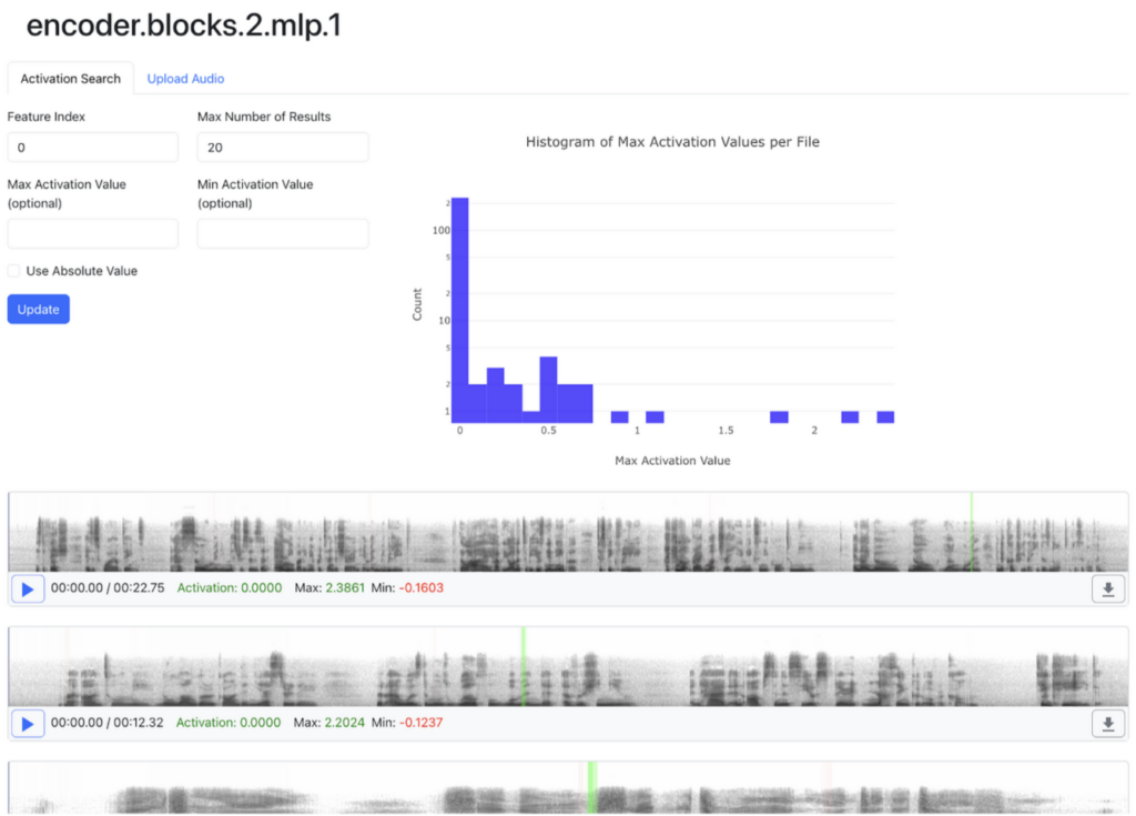
Search results for the audio files containing the strongest activations for index 0 of Whisper `tiny`’s block 2 MLP intermediate activations. The green bars indicate the position of strongest activation, corresponding to the “m” phoneme. 

Hurray! We did it. Interpretability is solved.

… but are these features really encoded linearly?

Let’s see what happens when we instead look at strong negative activations by setting max activation value to 0 and checking “Use Absolute Value”. If MLP indices linearly encoded phonetic features, we’d expect to see strong positive activations to correspond to the definite presence of a particular phoneme, and strong negative to correspond to absence. However…

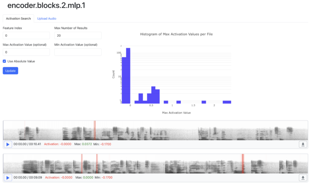
Search results for the audio files containing the strongest negative activations for index 0 of Whisper `tiny`’s block 2 MLP intermediate activations. The red bars indicate the position of strongest negative activation: like the strongest positive activations shown above, they correspond to the “m” phoneme. So, scaling the “feature vectors” given by MLP indices doesn’t correspond to our notion of what scaling a feature vector should look like semantically.

Moreover, Section 1.3 of Interpreting OpenAI’s claims that even positive activations for the MLP neurons exhibit polysemanticity, activating for qualitatively different phonemes at different scales. I tried replicating the linked result for the neuron at neuron 1 of block.2.mlp.1:

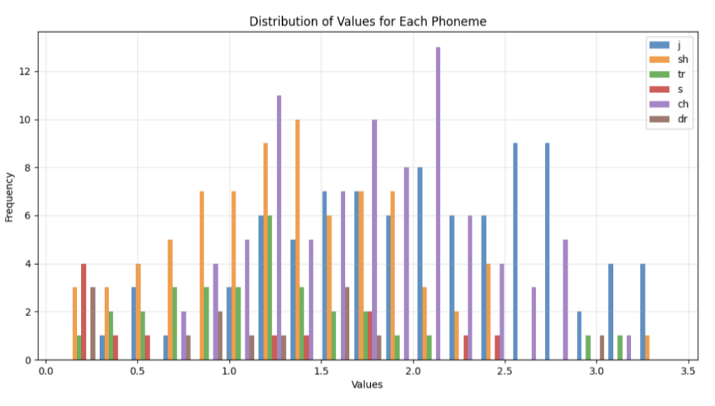
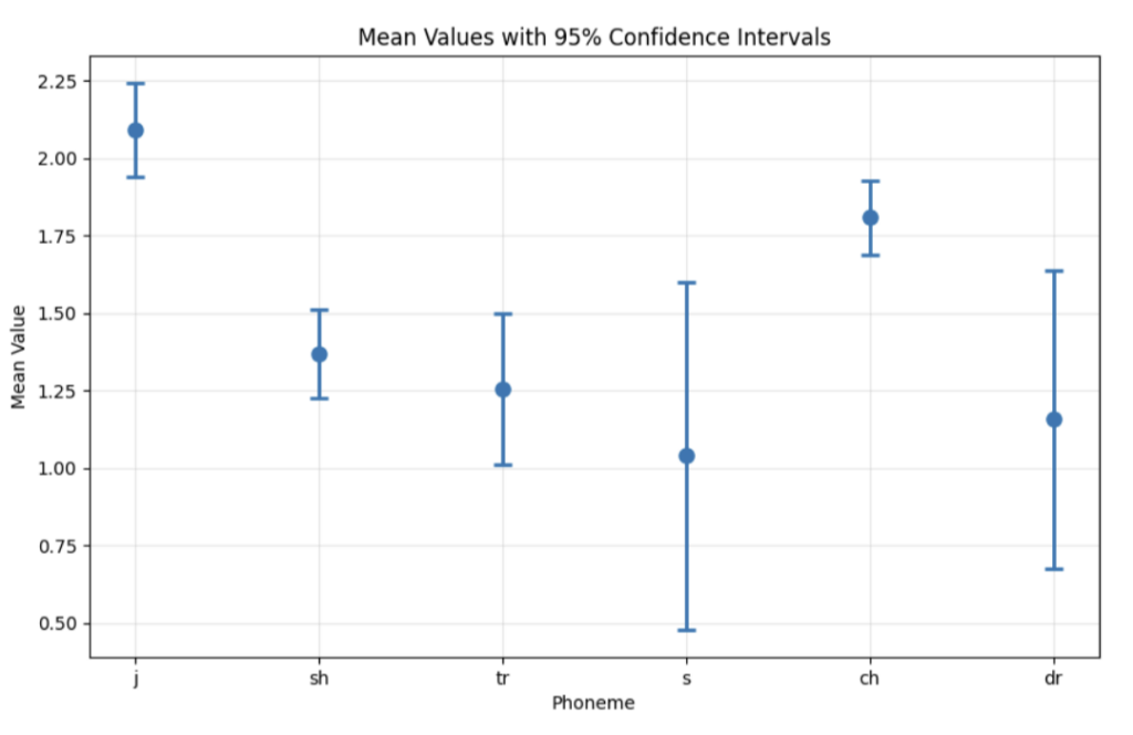
I find this result less damning of this MLP neuron linearly corresponding to a single phonetic feature since sh/tr/s/ch/dr all sound kind of like “j” and this would fit the hypothesis of high activation values for index 1 corresponding to near-certainty of “j,” and lower-but-still-nonzero values corresponding to lower certainty.

Let’s continue our observation of neuron 1 values into the negatives:

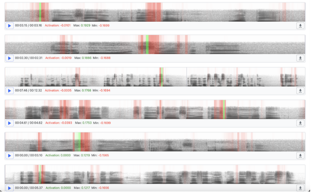
Isolated negative activations tend to correlate with “s” sounds, but occasionally “r” and “t” sounds. Moreover, we see an interesting “positive bookended with negative” activation pattern that only becomes visually distinct when the visualization code scales negative activations relative to comparatively sized positive activations. However, if we inspect manually, we’ll notice negative activations in the -0.17 to -0.15 range bookending strong positive activations, too. This odd “bookending” behavior is stronger evidence of nonlinear feature encoding to me.

Thus doubts have been sown that MLP neurons provide the linear decomposition of Whisper’s logic that we crave. Moreover, the layers without a preferred basis are also doing some computational work that warrants analysis. In part II, we use sparse autoencoders to analyze the residual stream of Whisper tiny’s encoder, scale up to larger Whisper models, and look at the representation of non-speech features.

Difficulties of analyzing other layers

There are two issues with trying to apply the naive “pick an index and look for correlated features” approach to all of Whisper’s intermediate activations:

1. No privileged basis: as previously discussed, only nonlinear transformations force features to align with a particular basis, since linear transformations will yield the same results if the basis is rotated before or after transformation
2. Feature superposition: I briefly talked about polysemanticity in the context of MLP neurons activation corresponding to different phonemes at different scales. Research from Anthropic argues that polysemanticity is a consequence of neural networks attempting to represent more features than there are neurons.

Suppose we wanted to construct a dictionary that mapped activation patterns to features. In that case, we’d have to start by going through a bunch of example activation data, learning common patterns, and then checking if those common patterns match features in the input. 

A neural network “going through a bunch of data and learning common patterns” was exactly what got us into this messy interpretability situation to begin with — but now, we’ll train a different kind of neural network to try to get ourselves out of it.

Sparse autoencoders

Autoencoders learn to take input data, encode a representation of the input, and then decode the representation back to the original data. The idea is that the encoding will have some desirable property that the raw input data lacks: maybe you want to produce a compressed representation of the input or embed the input into a linear space due to aforementioned nice properties of linear spaces. The decoding step keeps the network honest by ensuring that the encoded representation can be meaningfully said to contain the same information as the input.

In our case, we want an encoding that addresses the two complaints above:

1. Each index of the encoding should correspond to at least one meaningful feature
2. Each index of the encoding should correspond to no more than one meaningful feature

So we want an encoding that “unpacks” the superimposed features, granting each its own index. Our best candidate is a sparse autoencoder, trained with the dual objectives of minimizing reconstruction error and minimizing the number of encoder indices active per encoding (to ensure that encodings of relevant features get assigned specific indices rather than getting smeared across multiple). Here’s what the simplest architecture would look like:

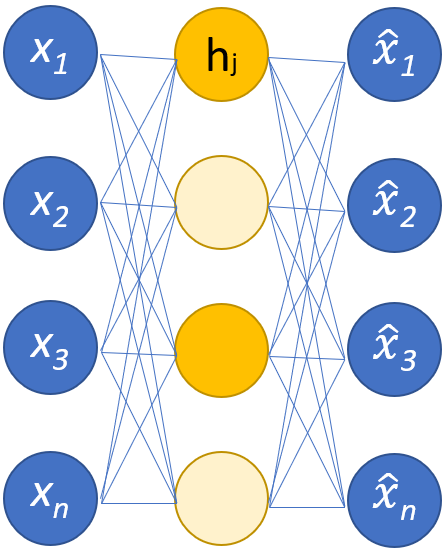
If this were a sparse autoencoder for Whisper activations:

• The leftmost column of blue nodes would represent an intermediate activation given as input to the network
• The middle column of yellow nodes would represent the encoding. Only a subset of the nodes (those in bright yellow) would be active for this specific input. Our hope is that these nodes consistently correspond to the same audio features across different inputs.
• The rightmost column of blue nodes would represent the reconstruction of the intermediate Whisper activation from the encoding. We could substitute this reconstructed encoding for the original intermediate activation to test the reconstruction’s faithfulness by observing how the substitution affects the Whisper model’s final output. Even more interestingly, we could perturb the encoding by turning some node’s activation way up or way down and then observe if substituting the activation reconstructed from the perturbed encoding produces output that reflects the feature associated with that node, i.e turning up a feature associated with the “l” phoneme produces a transcript that contains the word “log” in place of “dog”.

Previous work on sparse autoencoders

Sparse autoencoders have seen great success as a method for interpreting and even steering LLM output. Neuronpedia hosts autoencoders trained on various models and GUIs for interacting with the learned features. OpenAI used sparse autoencoders to interpret GPT-4, whose features you can browse here. 

Most entertaining has been Anthropic’s decision to demo their sparse autoencoder trained on Claude 3 Sonnet by turning up the encoding for a feature that they found to correspond to mentions of the Golden Gate Bridge, resulting in a model that tries to insert references to the landmark into every conversation:

Sparse autoencoder research has focused on text models not only because LLMs exhibit the most impressive (and mysterious) examples of complex reasoning across all domain-specific transformer models but also because we can use LLMs to automate the process of assigning input features to encoding indices, a process known as “autointerpretability”. 

First proposed by OpenAI for analyzing MLP neuron activations, autointerpretability involves giving a large “explainer model” examples of input corresponding to high activations at a particular index and asking for a hypothesis about what the inputs have in common. This summary is then fed to a “simulator model” that uses the hypothesis to generate inputs that can be fed back into the original model to determine how well they activate the index under investigation. This technique allows for proposed features to be analyzed at a greater scale and more efficiently than you’d get from human analysis.

Image and audio analysis and generation capabilities currently lag behind text, making autointerpretability challenging to implement for other modalities (maybe after the next generation of multimodal models)? Nevertheless, manual inspection of sparse autoencoders features yields interesting results for vision transformers, and the same research that we checked MLP neuron results against in the previous post also trained a sparse autoencoder on Whisper tiny’s block 2 residual stream. Let’s see what we can learn by replicating this work.

Analyzing L1-regularized autoencoder for Whisper tiny

L1-regularized autoencoders encourage sparsity by using the L1-norm of the encoding as a loss term, thus incentivizing the network to minimize the number of non-zero entries in the each encoding vector.

You can download a pretrained checkpoint here. After setting up the FREUD repo, start a server for the checkpoint:

python -m src.scripts.gui_server --config pretrained/l1auto encoder_baseline/features.json

and follow the instructions at General Note 3 to view the GUI (you can also run the collect_features script to cache activations to disk before running the gui_server script with the --from_disk flag). Your browser will display a GUI that looks like MLP feature demo, but with the title encoder.blocks.2.

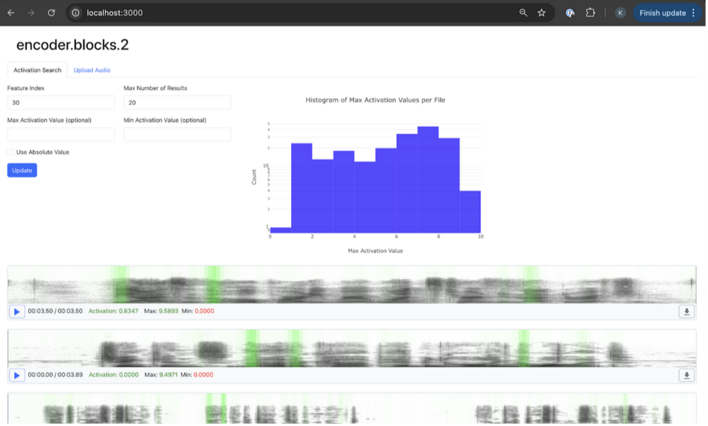
This training config gives us only 200 encoder dictionary entries, which probably isn’t enough to assign each relevant feature its own delineated entry. Indices tend to activate on a combination of similar-sounding phonemes. Some indices that I looked at, along with the strongest-activating phonemes:

• 85: m
• 101: ch/sh
• 166: i

Occasionally, I encounter a structural feature like 17, which activates on the boundaries between different words, even if there isn’t silence between them.

Let’s try something like the feature-manipulation trick that Anthropic used to create Golden Gate Claude. If you search for top activations for feature 30, you’ll notice that it seems to correspond to “th”. Now switch to the “Upload Audio” tab and upload pretrained/example_audio/8280-266249-0065.flac. Set the ablation factor for feature 30 to -1.

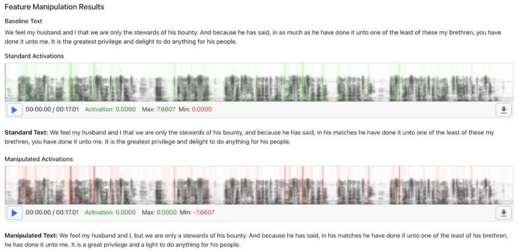
Notice how turning down feature 30 eliminates “th” in several parts of the transcript!

TopK autoencoder

Gao et al. (2024) introduce two innovations in sparse autoencoder training

• Rather than using L1-norm for loss, the autoencoder architecture forces all but the top k entries to 0 for each output.

• An auxiliary loss function that attempts to address the problem of “dead latents”:

“In larger autoencoders, an increasingly large proportion of latents stop activating entirely at some point in training. For example, Templeton et al. (2024) train a 34 million latent autoencoder with only 12 million alive latents, and in our ablations, we find up to 90% dead latents when no mitigations are applied (Figure 15). This results in substantially worse MSE and makes training computationally wasteful.”

I’ve found that L1-regularized autoencoders tend to have lower reconstruction error, though TopK autoencoders result in more stable training: L1-regularized runs for the Whisper-AT inspired experiment below would inevitably collapse into NaNs, while TopK runs converged. I’ve provided a pretrained checkpoint for a TopK autoencoder on Whisper tiny here.

Even with the aux-k loss, this checkpoint has many dead features, as you’ll discover if you randomly input feature indices into the GUI. Here are some non-dead features that I found:

• 0: w
• 2666: m
• 4985: r
• 3855: p/b
• 2523: mic or mouth noise
• 5155: a

Scaling up

Whisper large-v3 is the largest and most accurate member of the Whisper family. Will it yield more complex features?

You’ll find the checkpoint for a pretrained L1-regularized SAE for this model here. Loading it into the GUI, we’ll see phonetic features:

• 35568: t/d
• 3361: s
• 29673: you
• 17956: I

and some positional features:

• 16226: noise at start of recording
• 87: start of speech after a period of silence
• 36618: silence before speech

Here’s an interesting one. 7744 activates on spaces between words, but specifically spaces where you’d expect a comma. Uploading pretrained/example_audio/8280-266249-0065.flac and turning 7744 up by a factor of 100, we see an the transcript suddenly acquire lots of commas:

If you want to run your own experiments on other models in the Whisper family, just set the whisper_model name in the training config to any of the models mentioned here.

Looking for background noise features

It would be reasonable to suppose that intermediate speech-to-text model activations wouldn’t preserve information about background noise in the input audio. Background noise won’t make it into the final transcript; omitting it leaves more room to encode features directly relevant to speech content. 

However, Gong et al. (2023) discovered that Whisper large-v1 preserves background information into the deepest layers of the network. They proved this by training a linear layer on the output of Whisper’s final MLP layer. I attempted to achieve similar results by training a TopK sparse autoencoder on the residual of the middle block. You can see the checkpoint for that experiment here.

Following Gong et al.’s example, I trained on the AudioSet dataset and searched for features over ESC-50. Here are some classes that I discovered:

• 0: full-spectrum noise, particularly in outdoor settings
• 5098: laughter
• 1750: animal bleating, human laughter, bird calls
• 5713: sirens, animal and infant cries
• 9077: keyboard clacking
• 5713: sirens, animal and infant cries
• 7186: pause after a repeated sound
• 10170: coughing and infant cries
• 6374: silence before a sound
• 2641: coughing, laughter, sneezing
• 17967: bells, buzzing, honking
• 9823: bird and insect calls

SAE limitations

Sparse autoencoders limit us to analyzing activations on a per-layer basis, with no way of understanding how information flows between layers. Transcoders learn to represent MLP layers as linear transformations, which makes it possible to take a “pullback” of a later-layer feature in order to see what early-layer features cause the late-layer feature to activate.

Apart from that, sparse autoencoders suffer from a host of complications including feature absorption (when autoencoder entries “steal” tokens from co-occuring entries, resulting in strange holes in otherwise-interpretable features), dataset dependence and limited ability to transfer between base and fine-tuned models.

For these reasons, sparse autoencoders probably won’t be the final solution for mechanistic interpretability, but they’re pretty interesting to think about right now.

Future work

I didn’t perform exhaustive hyperparam sweeps for the checkpoints that I’ve provided, so it’s likely that other configs could produce better-delineated features and fewer dead latents. My code is also limited to Whisper family models, though it would also be interesting to analyze other popular speech-embedding models like HuBERT and wav2vec2. Hit me up over email, fork or open a PR if you’d like to share your own checkpoints or add features.